Measurement in Quantum Circuits: How Quantum Computers Extract Results
📖 10 min read | 2 Jun 2026 | Written by G Siva Prakash
Before measurement, a quantum computer holds infinite possibilities. After measurement, it gives you a single answer. Understanding what happens in between is the key to understanding quantum computing itself.
Introduction
When I first started researching quantum circuits, I kept running into the same wall. I could understand, at least loosely, how qubits work and what quantum gates do. But I kept asking: how does any of this produce a result I can actually read? The answer, I eventually found, is measurement, and it is far more interesting than the word suggests.
Measurement in quantum circuits is the process that converts quantum information into classical information of the ordinary 0s and 1s that computers, screens, and humans can actually use. Without measurement, all of a quantum computer’s extraordinary calculations exist in a kind of mathematical fog. Useful to no one.
What surprised me most during my research was that measurement is not just the final step of a quantum circuit. It is the bridge between the quantum world and the classical world we interact with every day. And the physics that governs it is genuinely strange in a way that changes how you think about information itself.
// Direct Answer
Measurement in quantum circuits is a process of extracting classical information from a qubit. It collapses the qubit’s quantum state into a definite 0 or 1, and that result is stored in a classical register for the user to read.
What Is Measurement in Quantum Circuits? for beginners
Defining Quantum Measurement in simple terms
In everyday life, measuring something is passive. You hold a ruler up to a plank of wood, and the plank does not care. Quantum measurement is completely different. When you measure a qubit, you fundamentally disturb it. The act of observing forces the qubit to choose a definite state, and it cannot go back.
This is one of those concepts that sounds simple but carries enormous depth once you sit with it. My understanding after researching this is that measurement is what makes quantum computations meaningful, it allows us to observe and interpret quantum states that would otherwise remain entirely hidden.
Why Measurement Is Necessary to Understand simply
A quantum computer runs calculations in a superposed, probabilistic state. But the output of any useful program, whether it is factoring a number, finding a molecule’s energy level, or searching a database, must eventually be a concrete result. Measurement is the mechanism that extracts the result. Without it, quantum circuits are technically executing but producing nothing observable.
Quantum Information vs Classical Information
In classical computers, information is stored as bits, definite 0s and 1s. Quantum computers operate on qubits, which can encode far richer information through combinations of states. The catch is that this richness is only available during computation. The moment you measure, the qubit collapses to the classical bit. You gain a concrete answer, but you lose the quantum state permanently. Read the difference between a classical vs quantum computer
QUANTUM WORLD
Superposed · Probabilistic
Rich · Hidden
MEASUREMENT
Collapse · Observe
Wave function → bit
CLASSICAL WORLD
Definite · Readable
0 | 1
Understanding Quantum States Before Measurement
The |0⟩ and |1⟩ States
A qubit’s two most basic states are written as |0⟩ and |1⟩. The quantum equivalents of classical 0 and 1. But these are not the same as classical bits. They are quantum states, meaning the qubit is not passively sitting in one position; it is actively existing in a mathematical space where both are possible simultaneously.
Superposition: The Core Idea
When I first studied quantum states, I found it genuinely surprising that a qubit can exist in multiple states before measurement. This is called superposition. Imagine a coin spinning in the air, it is not heads yet, not tails yet. It is in a superposition of both. The moment it lands (or you catch it), it becomes one or the other. A qubit in superposition is exactly that spinning coin. Measurement is the landing.
Probability Amplitudes Explained Simply
Before measurement, a qubit’s state is described by two numbers called probability amplitudes. These are not probabilities directly; they are something deeper. When you square them, you get the actual probabilities of measuring 0 or 1. A qubit with equal amplitudes for both states has a 50% chance of collapsing to 0 and a 50% chance of collapsing to 1. The amplitude carries phase information that probabilities alone cannot capture, which is what allows quantum circuits to perform interference and computation.
How Measurement Works in a Quantum Circuit
My research showed that measurement is often represented as a deceptively simple symbol in a circuit diagram, a little meter icon, yet it fundamentally and irreversibly changes the state of a qubit. Here is what actually happens, step by step.
Prepare the Qubit
Every circuit starts by initialising all qubits to a known state — almost always |0⟩. This is the clean starting point, the equivalent of clearing a whiteboard before writing.
Apply Quantum Gates
Gates rotate and entangle qubit states. A Hadamard gate (H) places a qubit in equal superposition. CNOT gates create entanglement. These operations encode the computation.
Perform Measurement
The measurement operator interacts with the qubit and forces it to collapse. The outcome, 0 or 1, is random, governed by the Born rule. The quantum state is destroyed.
Store Result in Classical Register
The classical outcome is written into a classical bit register — a memory cell that can be read by software, displayed on a screen, or used in further classical computation.
Measurement Probabilities and the Born Rule
Why Quantum Measurements Are Probabilistic
One thing I learned that genuinely shifted my thinking: quantum computers do not always produce the same result from a single run. This is not a bug. It is fundamental. A qubit in superposition does not have a hidden predetermined value waiting to be revealed; the outcome is genuinely undetermined until measurement occurs. This is one of the deepest and most debated aspects of quantum physics.
The Born Rule, Explained Simply
The Born rule is an equation that connects quantum amplitudes to measurement probabilities. In plain terms: if a qubit’s amplitude for |0⟩ is α and its amplitude for |1⟩ is β, then the probability of measuring 0 is |α|² and the probability of measuring 1 is |β|². These two probabilities always sum to 1; you always get one or the other. The Born rule is not derived from anything deeper in standard quantum theory; it is a foundational postulate that is simply confirmed, over and over, by experiment.
| Qubit State | P(measure 0) | P(measure 1) | Example |
|---|---|---|---|
| |0⟩ | 100% | 0% | Definite classical 0 |
| |1⟩ | 0% | 100% | Definite classical 1 |
| Equal superposition (H|0⟩) | 50% | 50% | Fair coin flip |
| Biased superposition | 25% | 75% | Weighted coin |
Because of this probabilistic nature, quantum circuits are typically run hundreds or thousands of times, called shots. The distribution of results across all those shots reveals the underlying probability structure, which is the real answer the algorithm is computing.
Wave Function Collapse During Measurement
While researching this topic, I found wave function collapse to be one of the most fascinating and philosophically contested concepts in all of physics. The basic idea is clean, even if the implications are deeply strange.
What Happens During Collapse
Before measurement, a qubit’s state is described by a wave function — a mathematical object encoding all possible outcomes and their amplitudes. The moment measurement occurs, this wave function collapses. The qubit is no longer in a superposition of states. It is in one definite state, and that state is what gets recorded.
What beginners often misunderstand is that collapse is not just a change in our knowledge of the qubit — it is a physical change in the qubit itself. Before measurement, the qubit genuinely exists in superposition. After measurement, the superposition is gone. This is experimentally verified and is not just an interpretation.
Measurement Bases in Quantum Circuits
What Is a Measurement Basis?
I discovered something during my research that most beginner articles skip entirely: you can actually choose how you measure a qubit. The standard measurement — the Z-basis — gives you 0 or 1. But there are other bases, and each one reveals a different aspect of the qubit’s state.
The Computational (Z) Basis
This is the default. Measuring in the Z-basis collapses the qubit to either |0⟩ or |1⟩, which directly corresponds to classical 0 and 1. Almost all basic quantum circuits use this basis by default.
X-Basis Measurement
To measure in the X-basis, you apply a Hadamard gate before the standard measurement. This reveals whether the qubit was in a |+⟩ or |−⟩ state — the superposition states that the Z-basis cannot directly distinguish. Changing the measurement basis is like rotating your viewpoint to see a different dimension of the quantum state.
Computational Basis
Hadamard Basis
Phase Basis
Why does this matter? Because choosing the wrong basis is like trying to read text with the wrong glasses — you will get a result, but it will not tell you what you actually wanted to know. In protocols like quantum key distribution, basis selection is the entire mechanism of security.
Measurement of Entangled Qubits
During my research, I found that entangled qubits produce measurement results that simply cannot be explained using classical intuition alone. This is the part of quantum measurement where the story becomes genuinely strange.
What Entanglement Does to Measurement
When two qubits are entangled, their states are not independent. Measuring one qubit instantly determines the outcome of measuring the other — regardless of how far apart they are. The most famous example is the Bell state, where measuring the first qubit as 0 guarantees the second will also be 0, and measuring the first as 1 guarantees the second will be 1.
This is not like pulling a pre-sorted pair of gloves out of separate boxes and realising they match. Experiments — confirmed through decades of Bell test experiments — show the correlations are stronger than any pre-sorting could explain. Entanglement is a genuinely quantum form of correlation with no classical equivalent.
Mid-Circuit Measurement and Dynamic Quantum Circuits
I learned something during my research that I did not expect: measurements do not always happen at the end of a quantum circuit. Modern quantum processors can perform measurements while the computation is still running — and then use those results to decide what to do next. This is called mid-circuit measurement, and it changes what quantum computers can do.
What It Enables
In a standard circuit, all gates run, then measurement happens at the end. In a dynamic circuit, a mid-circuit measurement produces a classical bit, and that bit can control which gates are applied to the remaining qubits. This is called a conditional operation. It is similar to an if-statement in classical code, except it is happening during a live quantum computation.
Mid-circuit measurement is essential for quantum error correction — where errors are detected and corrected without collapsing the main computation. It is also central to quantum teleportation protocols and more efficient implementations of quantum algorithms. IBM’s quantum processors have supported mid-circuit measurements since 2021, and it is a significant step toward genuinely useful quantum hardware.
Measurement Errors and Practical Challenges
One important insight from my research is that measurement itself introduces inaccuracies, making error mitigation an essential, not optional, part of practical quantum computing. This surprised me. I had assumed errors came from gates and noise during computation. But the readout process itself is a significant source of error.
Readout Errors
Readout errors occur when a qubit is actually in state |0⟩ but the measurement equipment reports a 1, or vice versa. On current hardware, these errors range from about 0.5% to several percent per qubit. They accumulate across many qubits and many shots, quietly corrupting the probability distribution that your algorithm relies on.
Error Mitigation Techniques
Several techniques help fight measurement error without requiring full quantum error correction. Readout error mitigation uses a calibration matrix built by measuring known states — then mathematically inverting the error to recover the true distribution. Zero-noise extrapolation runs the same circuit at artificially increased noise levels and extrapolates backward to the ideal zero-noise result. These are software solutions running on top of noisy hardware, and they work surprisingly well.
Readout Errors
Decoherence During Readout
Error Mitigation
Repeated Shots
Applications of Measurement in Quantum Algorithms
I found that every useful quantum algorithm ultimately relies on measurement to transform quantum computations into actionable results, and the way measurement is used varies significantly depending on the algorithm.
Quantum Search (Grover's Algorithm)
In Grover’s algorithm, the circuit amplifies the probability amplitude of the correct answer through a series of reflections. A single measurement at the end has a high probability of landing on the correct solution — made possible by carefully orchestrated interference before the measurement occurs.
Variational Quantum Algorithms (VQAs)
Algorithms like the Variational Quantum Eigensolver (VQE) run a parameterised circuit, measure the result, use that measurement to calculate an energy expectation value, and then adjust the parameters using a classical optimiser. This loop repeats until the energy converges. Measurement here is not the final step — it is inside a classical-quantum feedback loop.
Quantum Error Correction
Error correction codes like the surface code use syndrome measurements — carefully designed mid-circuit measurements of ancilla qubits — to detect errors in the data qubits without collapsing them. The classical processor interprets the syndrome and applies corrections. It is the most measurement-intensive use of quantum hardware, and the key to fault-tolerant quantum computing.
Best Practices for Interpreting Quantum Measurement Results
Run Enough Shots
Single-shot results are almost meaningless for probabilistic circuits. Use 1,000–10,000 shots to get a stable probability distribution unless you are running a deterministic algorithm with a known outcome.
Choose the Right Measurement Basis
Default Z-basis works for most algorithms, but if you are probing phase relationships or running quantum state tomography, you need to measure in multiple bases and combine the results.
Apply Readout Error Mitigation
On real hardware, always calibrate for readout errors. Most quantum cloud platforms (IBM Quantum, Google Cirq, Amazon Braket) offer built-in readout mitigation options. Use them.
Validate Against Simulation
Before running on real hardware, simulate on a noiseless backend. Compare the ideal distribution to the noisy hardware distribution — the gap tells you how much noise is affecting your result.
Key Takeaways
- Measurement converts quantum information into classical information — it is the only way to extract a usable result from a quantum circuit.
- Quantum measurements are probabilistic, not deterministic. The Born rule governs the probabilities from amplitude values.
- Wave function collapse is irreversible — once a qubit is measured, its superposition is permanently destroyed.
- The measurement basis determines what information you extract — different bases reveal different aspects of the qubit’s state.
- Entangled qubits produce correlated measurement outcomes that cannot be explained classically.
- Mid-circuit measurement enables dynamic circuits where classical measurement results control subsequent quantum operations.
- Readout errors are a real and significant source of noise on current hardware — error mitigation is essential.
After researching measurement in quantum circuits, I came to understand that it is far more than a final step in a quantum computation. The whole enterprise of quantum computing — from designing algorithms, to managing errors, to extracting useful answers — is built around the constraints and possibilities that measurement imposes.
Every qubit’s rich quantum state exists only until you look at it. That single fact — that observation changes what is observed — is what makes quantum computing so different from anything that came before. And learning to work with that constraint, rather than against it, is what makes quantum algorithms so clever.
“After researching measurement in quantum circuits, I came to understand that measurement is far more than a final step. It is the process that connects quantum phenomena with observable outcomes — the moment where the quantum world speaks in a language we can finally understand.”